Inferring Stock Price Distribution from Option Quotes
Exploring going from Option Quotes to a probability distribution of the price of the underlying at expiry.

It is no secret that options and the underlying instruments are very intimately related and movements in options markets are highly influenced by the movements in the underlying market. In particular, we know that options are forward looking, as they are essentially bets on the future prices of the underlying. Therefore, it seems natural to think that option quotes give some notion of what the market thinks the price of the underlying is going to be at expiry. In particular, it would be useful to know what the consensus expectation of the underlying price at expiry is, based on how the options are priced, as that could result in several arbitrage trades or trades that compare the consensus price and our forecasted price.
The Pricing of Options
A call option is defined as the right (but not obligation) to buy the underlying instrument at a predefined price (known as the strike price) at a future date (known as the expiry date). Similarly, a put option is defined as the right (but not obligation) to sell the underlying at a strike price at expiry.
Logically, the intrinsic value of an option would depend on what the price of the underlying is going to be at expiry. A call (put) option would therefore only payout if the underlying price is higher (lower) than the strike at expiry. This naturally leads us to define a few useful terms: an In the Money (ITM) option is an option whose strike such that if I were to exercise now, I would have a net profit. An Out of the Money (OTM) option is when the strike is such that if I were to exercise now, I would be at a net loss. At the Money (ATM) options are when strike equals underlying price now. We can now make an important inference about the value of an option: the option would be more valuable if it was ITM than if it was OTM.
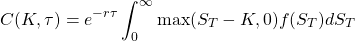
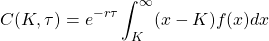
If we attempt to make this more concrete, by the no arbitrage argument, the fair value of the option is the expected payout of the option at expiry, discounted by the risk-free rate till expiry, or mathematically

where K is the strike, tau is the time between now and expiry, r is the risk-free rate and S_T is the price of the underlying at expiry. In order for us to find the fair price of the option using that formula, we need to know what the expected payout is going to be. In other words, we need to know what the distribution of the price of the underlying is going to be at expiry. One way we can do that is if we had a probability distribution function for the price of the underlying at expiry. Obviously, that is not a trivial task, so we are going to have to make some assumptions.
Black-Scholes Pricing
In this section, we build upon our fair value formula and find a way to solve for the value of the option. The main assumptions of the Black-Scholes Model (BSM) are
No arbitrage opportunities
Log Returns of prices are normally distributed (in other words, the stock price follows a Geometric Brownian Motion, with constant drift and volatility)
Risk free rate is constant
No dividends in the period of analysis
No transaction costs
Given these assumptions, we can solve for the expected payout of an option at expiry. Furthermore, by using Feynman-Kac formula, we can convert the stochastic process that gives the expected payout into a partial differential equation of the following form
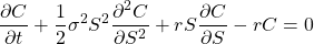
Without going into the technical details of solving the BSM, we just need to understand a few key points, mainly that there is an intimate relationship between the options fair value and the distribution of prices of the underlying at expiry. This therefore in a way motivates our whole discussion.
Relating Price Distribution to Option Quotes
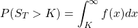
Coming back to our original question, we now have a semblance of an idea on how to approach formulating a distribution of prices. Firstly, let us define our probability distribution function (PDF) for the prices of the underlying at expiry to be f(x). So now we can write the probability that our underlying expires at a price higher than the strike as
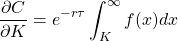
So now, if we want to calculate the fair value of the option
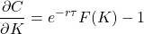
Now, if we differentiate this with respect to the strike, we obtain
If we then use the definition for a cumulative distribution function (CDF), we get
So now we differentiate with respect to K again, and finally get
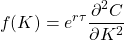
This result is known as the Breeden Litzenberger (BL) formula, which they derived in their 1978 paper.
Option Quotes
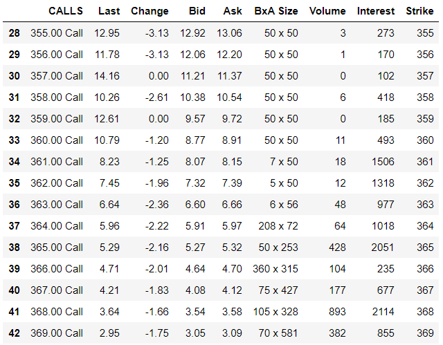
Historical options data are notoriously hard to find as a retail trader, so I got my option quotes from my broker. These are the option quotes for the 23/12/2020 expiry SPY options dated 09/12/2020 1915hrs GMT, with SPY price at 366.42.
The following is a scatterplot of the prices against the strikes for both calls and puts.
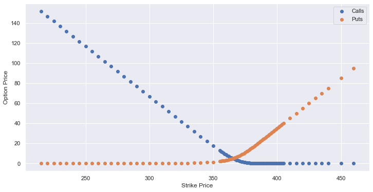
As we can observe, the granularity of the options decrease as the strikes get further away from the ATM price. This is going to pose some issues for us down the road when we try to find the implied distribution.
From our expression relating the probability distribution for the price of the underlying and the options prices, we know that our goal is to find the second derivative of the options prices with respect to quotes. In other words, we want to find the curvature of the curve plotted in Fig 1. In the following sections, we explore a few ways to do so.
Interpolating and Smoothing
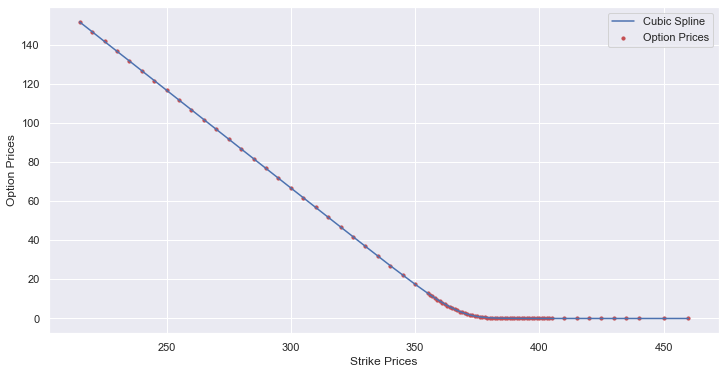
In order to find the curvature of the scatter plot, we can either do numerical differentiation on the actual datapoints or we can perform some form of interpolation and then find the curvature of the interpolated function. The issue with the former approach would be the lack of data, and large spacings between strikes in the deep ITM options, which would make numerical differentiations undesirably inaccurate. Therefore, we are going to perform an interpolation of the data.
We are going to be using Cubic Splines to interpolate between the points and form a continuous function for our option value for various strikes.
Having interpolated our option prices, we can now use our BL formula to calculate the stock price pdf. We obtain the following pdf for our SPY price on 23/12/2020.
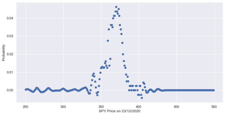
Although obvious, I think we need to point out a few issues with the pdf:
There are negative values!
High level of noise in the data
One workaround this would be to consider some form of smoothing and kernel density estimation. So first of, we can attempt to smooth out the noise in the pdf and to constrain the pdf to be nonnegative using a Gaussian Smoother. We then get the following pdf.
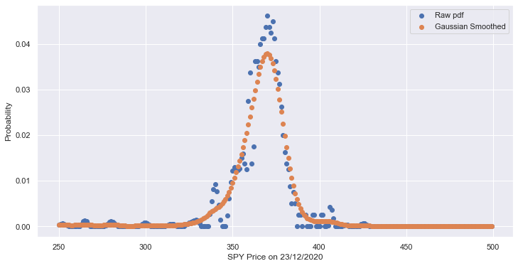
That looks much more reasonable, with minimal noise and no negative values. We can take this one step further to form a full probability distribution function by applying a gaussian kernel density estimator to find a nonparametric probability density for the SPY price.
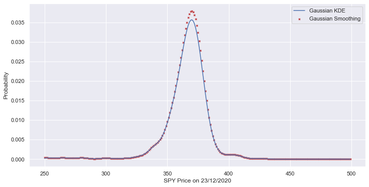
That pdf looks reasonable and there definitely are no major issues that affect the validity of the pdf of our SPY estimate on 23/12/2020.
Utilising the Volatility Space
Although our pdf estimation using options prices alone was acceptable, we can bypass the issues with negative probabilities and high levels of noise by looking into other parameters in the options pricing that might have a better fit. One parameter that springs to mind is the volatility of the underlying. Since we are trying to find the implied distribution of the price of the underlying, we can do the same with the implied volatility of the underlying. Implied volatility (IV) is the volatility ‘implied’ by the option prices. In other words, what volatility in the underlying instrument would give the current option prices. Mathematically, it is simpler to understand what IV is, as IV is essentially an inverse of the BSM from prices to volatility. Note that the estimation of IV is a heavily researched topic, and I am in no way an expert in the field.
In this case, we are going to stick to a simple Newton’s method to recursively calculate our IV. The method, being derived from the BSM, uses the same assumptions, which are stated in the first section. It results in the following volatility smile for our set of option quotes.
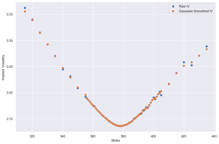
As before, the volatility smile has been smoothed using a Gaussian smoother in order to reduce the noise from the numerical estimation.
I think this deserves a detour. The volatility smile is a well researched phenomenon where the IV for the options that are deep ITM or OTM are much higher than the IV for options ATM. In the BSM, volatility is a constant parameter, and it describes the variance of the stock price in the geometric brownian motion assumption. Therefore, it is natural to predict that the implied volatility should remain constant as the underlying is the same. However, as we observe when we calculate our implied volatilities, the IVs are not constant, and we see a ‘smile’, so to speak, in the IV across the strikes. This is an indication of the invalidity of BSM at the deep ITM and OTM options. However, this does not mean that our BSM model is incorrect or is useless in application, as by being wary of the effects of IV smile, we can account for the inaccuracy in the BSM. We can note the following about index option IVs:
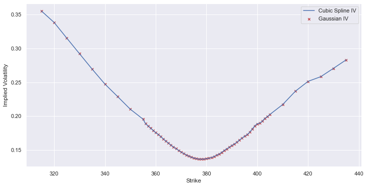
A very noteworthy characteristic would be the negative slope of the IV as a function of the strikes. As seen from Fig 7, this slope becomes less steep as the strikes increases from far ITM to ATM, with higher IVs at lower strikes compared to higher strikes. This can be attributed to the fact that there are more large scale down moves than up moves. Over the course of the history of the SP500, there have been several 20% down moves in a day, but almost never has there been a 20% ‘upmove’ in a day. This is retrospectively depicted in the skew of the IV smile. Furthermore, the skew can be attributed to investors wanting to hedge their negative downsides by buying OTM options with the premium.
The negative skew of the IV with respect to the strikes is steeper for options with short expiries. Furthermore, unlike the strike structure of IV, the term structure can be either positive or negative, and it depends on prevailing market conditions. During market crises, the volatility is expected to be high and hence the term structure is downward sloping. The high short term volatility followed by lower long term volatility reflects the view that the short term volatility will result in the market returning to ‘normal’ levels of volatility.
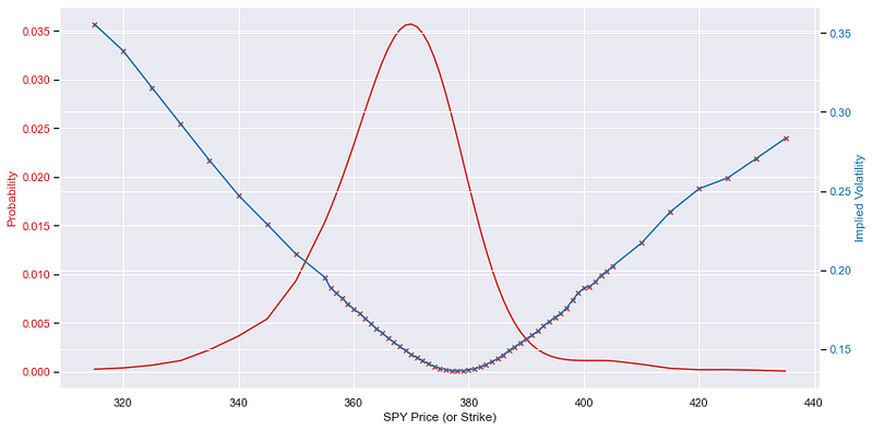
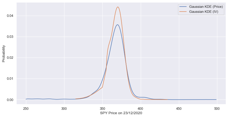
Coming back to the problem of finding the PDF of the price distribution, we can now compare using the option quotes versus using the IV smile to estimate the distribution. As evident from the Fig 8 below, we can conclude that the distribution is similar, but with the IV estimation having a smoother pdf.
Conclusion
We have briefly explored how to use option quotes to infer a probability distribution for how the underlying is going to move at expiry. However, it is an ever evolving topic and we have plenty of avenues to explore. For example, we can use the put prices to generate more call price data, perhaps using the put-call parity. Furthermore, we can adopt a parametric model for the volatility surface, especially if we have more data for the term structure of the IV (I am limited by the data available to me), and that would allow for some interesting extensions where we consider the change in the distribution of the underlying over a period of expiries. These extensions are something I am looking to explore, especially if I can get my hands on some options quotes for various expiries.